Large Language Models (LLMs) are everywhere and are substantially changing the way we perform many daily tasks. Recently, I noticed a growing number of positions related to the post-training of such models. Interestingly, two aspects consistently caught my attention: most of them were related to 1) computational efficiency and 2) Reinforcement Learning. At the same time, many of the companies announcing these positions did not appear to have computational resources remotely comparable to those of frontier labs capable of training multi-billion-parameter models from scratch. Clearly, something interesting was going on. That curiosity led me to investigate, for the very first time, how modern LLMs actually work.
To illustrate some of the concepts I learned during this process, we are going to use the GSM8K dataset (Cobbe et al. 2021). This dataset consists of question-answer pairs involving elementary mathematical reasoning problems. Although each individual operation is simple, solving the hardest examples often requires composing multiple arithmetic steps coherently. Let’s look at the following example:
{
  "question": "James writes a 3-page letter to 2 different friends twice a week. How many pages does he write a year?",
  "answer": "Each letter has 3 pages and he writes to 2 friends, so each session is 3 * 2 = 6 pages. He writes twice a week, so that is 6 * 2 = 12 pages a week. There are 52 weeks in a year, so he writes 12 * 52 = 624 pages a year. #### 624"
}
As the name suggests, GSM8K contains roughly $\sim 8k$ examples split across training and test sets. At this point, an obvious question emerges: if these problems are relatively easy for modern LLMs, where exactly is the challenge? Indeed, most recent frontier models would likely solve this dataset with near $100\%$ accuracy. However, the key point is that such models have already been trained on massive corpora collected from the internet and have almost certainly seen similar reasoning patterns during pretraining. In practice, companies often possess their own internal and non-shareable datasets containing proprietary workflows, product-specific knowledge, internal protocols, or business-sensitive information. Naturally, they do not want to expose such data publicly. At the same time, training a new foundation model from scratch would require an enormous computational investment.
The practical solution is therefore straightforward: start from a pretrained model and adapt it to the target domain through finetuning. In this article, we are going to cover how this process works in practice, including a brief discussion about Mixture of Experts (MoE) architectures, supervised finetuning with Low-Rank Adaptation (LoRA), and finally, post-training using Reinforcement Learning (RL).
Before moving forward, let us first understand what a Mixture of Experts (MoE) architecture is and why it enables strong performance while keeping computational costs manageable. MoE architectures were originally introduced in (Jacobs et al. 1991) and consists of simple idea: instead of using a single massive neural network, we divide the model into multiple smaller specialized subnetworks called experts. The key observation is that, during inference, not all parameters of a large model are equally necessary to process a given input. For example, in Natural Language Processing (NLP), different tokens or reasoning patterns may benefit from different specialized computations. Rather than activating the entire network for every token, MoE models dynamically route information through only a subset of experts at each step. This approach substantially increases the model capacity without proportionally increasing the computational cost during training and inference.
But how does the model decide which experts should process a given input? For this, MoE architectures employ a component called the router (also known as the gating network). Given an input $x$, the router assigns a probability distribution over the available experts ${e_1, \dots, e_n}$ and selects the top-$k$ experts according to these probabilities, where $k$ is a user-defined hyperparameter. The outputs of the selected experts are then combined through a weighted average:
$$ y = \sum_{i \in \tau} p_i(x)e_i(x) $$where $\tau$ denotes the set of selected experts and $p_i(x)$ represents the routing probability assigned to expert $e_i$. Since the router itself also contains trainable parameters, the routing strategy improves over time as the model learns which experts are more useful for different types of inputs. Intuitively, the objective is to encourage some experts to become better at processing specific patterns or domains, such as mathematical reasoning, code generation, or natural language understanding. There exist many sophisticated strategies to stabilize and optimize routing in MoE systems. However, the goal of this tutorial is simply to introduce the core ideas behind MoE architectures, since we are going to work with a pretrained MoE model rather than train one from scratch.
Next, let’s consider a highly resource-constrained scenario in which only a single GPU is available. In such settings, even relatively small pretrained models may become challenging to load due to VRAM limitations. To mitigate this issue, quantization is commonly employed. The intuition behind quantization is relatively simple: imagine continuous numerical values represented with high precision being discretized into a much smaller set of possible values. Naturally, this process sacrifices some numerical precision. However, neural networks are known to contain a significant degree of redundancy, which raises the hope that reducing precision will not substantially degrade performance. In practical terms, quantization typically converts parameters stored in formats such as float16 into lower-precision representations such as int8 or even int4, drastically reducing memory consumption and enabling larger models to fit within limited hardware budgets.
Although quantization substantially reduces memory consumption, our pretrained model still contains a massive number of parameters that are not specialized for the target task. This naturally raises the following question: instead of finetuning all weights of the pretrained model, what if we kept its original knowledge and only learned a small task-specific correction on top of it? This is precisely the idea behind Low-Rank Adaptation (LoRA). Rather than updating the pretrained weights directly, LoRA introduces a small set of highly trainable parameters (adapters) that learn how to refine the output of the frozen model using target-specific data.
LoRA was introduced by (Hu et al. 2022) and is based on two main hyperparameters: the rank $r$, which controls the size of the trainable adaptation, and $\alpha$, which scales the contribution of this adaptation to the final output. Formally, let $W$ denote the frozen pretrained weight matrix. LoRA introduces two trainable low-rank matrices, $A$ and $B$, such that the original transformation is augmented by a low-rank correction term. Given an input $x$, the adapted output $x’$ becomes:
$$ x' = xW + (xAB)\frac{\alpha}{r} $$where typically $A \in \mathbb{R}^{d \times r}$ and $B \in \mathbb{R}^{r \times k}$, with $r \ll d,k$. Intuitively, LoRA behaves as a lightweight deviation from the original pretrained pathway. Since only the adapter parameters are trained, the original model remains frozen, substantially reducing memory consumption and computational cost. An additional practical advantage is modularity: because the pretrained model itself is left untouched, different LoRA adapters can be swapped in and out for different tasks without requiring multiple copies of the full model.
As a final step, we would like to improve the reasoning capabilities of our model. To achieve this, Reinforcement Learning (RL) has increasingly been employed as a post-training stage for LLMs. Coming from an RL background, the first question that naturally comes to mind whenever someone mentions using RL is: what exactly is the task? Or, more formally, what is the underlying Markov Decision Process (MDP)? This question is important because once the task is properly defined, a wide range of RL approaches becomes available: online or offline methods, on-policy or off-policy algorithms, among many others. Regardless of the algorithmic choice, however, defining the MDP is fundamental.
Interestingly, the MDP formulation for LLMs is surprisingly straightforward. Given a prompt (initial state $s_0$), the agent (the LLM itself) begins generating tokens sequentially. Each generated token corresponds to an action, and each newly generated partial sequence defines the next state in the rollout:
$$ (s_0, a_0, s_1, a_1, \dots, s_t) $$The challenging part is not defining the states or actions, but rather assigning credit properly. If we reward every generated token equally, the model may learn undesirable behaviors such as producing unnecessarily long outputs or verbose explanations that do not actually improve the final answer. On the other hand, rewarding only the exact final output, for example, simply producing #### 624 in your previous example, makes it difficult to encourage interpretable reasoning or structured responses.
This tension motivated the emergence of RL from Human Feedback (RLHF). If you have used modern LLM systems before, you have probably encountered situations where the model presents two candidate answers and asks which one you prefer. In that moment, you are effectively providing a preference signal (or, in RL terminology, a reward signal) that can later be used to refine the model. However, recall that we are building our pipeline on top of a pretrained MoE model. Such models are already reasonably good at generating coherent language and structured reasoning traces. Our primary goal is therefore not teaching the model how to write, but rather improving its performance on the target task itself — in this case, elementary mathematical reasoning.
For this reason, we can leverage the pretrained linguistic capabilities of the model and focus the reward primarily on the correctness of the final answer. One possible reward function is:
$$ R = w_{\text{exact}} R_{\text{exact}} + w_{\text{format}} R_{\text{format}} $$where the term $R_{\text{exact}}$ represents the primary learning objective. It assigns reward only when the extracted answer exactly matches the ground-truth solution. This creates a highly sparse reward signal, but one that remains perfectly aligned with the evaluation metric we actually care about. Meanwhile, $R_{\text{format}}$ provides a small auxiliary bonus whenever the strict parser successfully detects a valid answer format. Importantly, this term is independent of correctness; its sole purpose is to improve answer extractability and reward reliability during training. Since the ultimate objective is exact-answer accuracy, here we deliberately favor a sparse but strongly aligned reward formulation, avoiding intermediate rewards that could unintentionally bias the model toward incorrect, yet numerically close, solutions. Finally, $w_{\text{exact}}$ and $w_{\text{format}}$ are tunnable weights, being expected that $w_{\text{exact}} \gg w_{\text{format}}$.
Now that the task is defined, let’s go through the final step of our model’s refinement: the RL post-training. With computational constraints in mind, even though only the LoRA adapters remains trainable, we gonna chose a simple but efficient algorithm for this task called REINFORCE with an exponential moving average (EMA) baseline. Given a prompt $x$ and a sampled completion $y$, the standard REINFORCE objective is:
$$\nabla_{\theta} \, \mathbb{E}[R(y)]= \mathbb{E}\left[ R(y)\,\nabla_{\theta}\log \pi_{\theta}(y \mid x) \right]$$where $R(y)$ is a scalar reward computed from the extracted final answer and $\log \pi_{\theta}(y \mid x)$ is the log probability of the entire sequence given the current policy $\pi$ parametrized by weights $\theta$. However, as mentioned, we actually employ a baseline to make the learning process more stable since the credit assignment is near-binary. Thus the baseline is calculated as:
$$ b_t = \beta \cdot b_{t-1} + (1 - \beta) \cdot R_t, $$where $\beta$ is a parameter and $R_t$ is the current reward average. Thus, the REINFORCE update at the timestep $t$ becomes:
$$\nabla_{\theta} \, \mathbb{E}[R(y)]= \mathbb{E}\left[ (R(y) - b_t)\,\nabla_{\theta}\log \pi_{\theta}(y \mid x) \right]$$This baseline algorithm corresponds to unbiased estimation when it is independent of the current sample and we can show this by expanding this expression:
$$ \hat{\nabla}_\theta J(\theta) = \mathbb{E}\left[ R(y) \nabla_\theta \log \pi_\theta(y|x) \right] - \mathbb{E}\left[ b \cdot \nabla_\theta \log \pi_\theta(y|x) \right] $$The first term is the original policy gradient. The second term can be rewritten as:
$$ \mathbb{E}\left[ b \cdot \nabla_\theta \log \pi_\theta(y|x) \right] = b \cdot \mathbb{E}\left[ \nabla_\theta \log \pi_\theta(y|x) \right] $$It is a fundamental property that:
$$ \mathbb{E}_{y \sim \pi_\theta(\cdot|x)} \left[ \nabla_\theta \log \pi_\theta(y|x) \right] = 0 $$Therefore, if the baseline $b$ is independent of the sampled trajectory $y$ (i.e., it does not depend on the current sample), the second term vanishes:
$$ \mathbb{E}\left[ (R(y) - b) \nabla_\theta \log \pi_\theta(y|x) \right] = \mathbb{E}\left[ R(y) \nabla_\theta \log \pi_\theta(y|x) \right] $$However, in practice, our moving average baseline is only approximately unbiased, but the reduction in variance makes it a very effective choice.
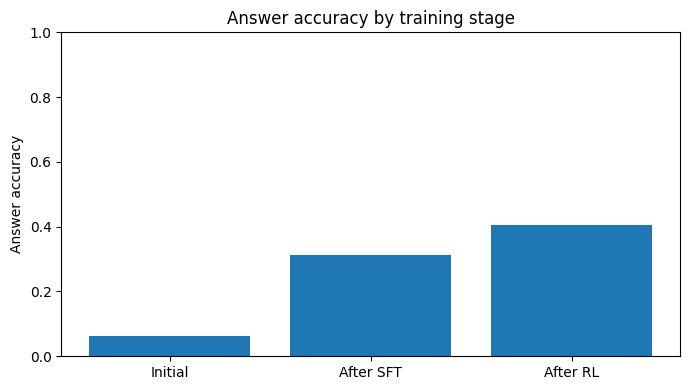
Now that our pipeline is completed, let’s analyse the results! Figure below shows how accurate the answers were at each step of the training pipeline. The “Initial” stage is when the pretrained MoE model is tested without any changes made to fit the task. In the “After SFT” stage, the model is fine-tuned with teacher forcing on task-specific samples and their correct answers. This gives a stable starting point for optimization later on. Last but not least, the “After RL” stage uses a REINFORCE-style policy gradient algorithm as a post-training step. In this stage, completions made by the model are sampled and improved based on the proposed reward function. Only 256 samples were used for training and 32 for testing in this experiment, along with the other hyperparameters that were given in the notebook to reproduce the results. The results indicate that supervised fine-tuning substantially improves performance over the pretrained baseline, while the subsequent RL stage further refines the model by aligning generation behavior with the evaluation objective.
Cobbe, Karl, Vineet Kosaraju, Mohammad Bavarian, Mark Chen, Heewoo Jun, Lukasz Kaiser, Matthias Plappert, et al. 2021. “Training Verifiers to Solve Math Word Problems.” arXiv Preprint arXiv:2110.14168.
Hu, Edward J, yelong shen, Phillip Wallis, Zeyuan Allen-Zhu, Yuanzhi Li, Shean Wang, Lu Wang, and Weizhu Chen. 2022. “LoRA: Low-Rank Adaptation of Large Language Models.” In International Conference on Learning Representations. https://openreview.net/forum?id=nZeVKeeFYf9.
Jacobs, Robert A., Michael I. Jordan, Steven J. Nowlan, and Geoffrey E. Hinton. 1991. “Adaptive Mixtures of Local Experts.” Neural Computation 3 (1): 79–87. https://doi.org/10.1162/neco.1991.3.1.79.